You all know how to use hash maps, hash tables, dictionaries and maps in programming languages. But what’s the mechanism behind the hash tables that provide O(1) for reading from and writing to it? Is it actually O(1) of time complexity or just a myth?

As you know, C is one of the best teachers when it comes to understanding how data structures work under the hood. Another fact about C is that there is no built-in data structure such as map. So we can write our own hash table implementation in C.

Before writing any code, we need to understand what we are talking about. Let’s explore what actually a hash table is and reveal the mystery behind this data structure.

Hash Table Concept

In hash tables, there are two main points:

1. hash function
2. buckets

You may have heard of hash functions already, so I won’t explain them in depth here. Buckets, as the name suggests, are where data is stored. Each hash table contains multiple buckets. In this implementation, each bucket is represented as a linked list.

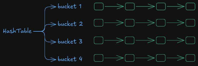
The relation of hash function and buckets

If you come up with the question: each bucket is a linked list, how is this linked list created and extended?, that’s a good question. This is where hash functions come into play. Hash functions are used to make series of bits out of a key and decide into which bucket we should place the key.

"a" -> hashfunc() -> 01011101 00111001 (23865)

Insertion

Suppose our hypothetical hash function accepts a string and returns 2-byte unsigned integer. Now you have a number derived from your string, and you can easily use the modulo operation to assign it to one of the buckets.

number_of_buckets = 4
hashed_value = hashfunc("a") // 01011101 00111001
selected_bucket = hashed_value % number_of_buckets

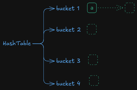
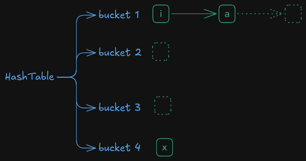
Note that it doesn’t matter whether your selected bucket has already keys or not, new keys will be inserted as the first node of the linked list.

Suppose i, x would be placed in bucket 1 and bucket 4 respectively:

Lookup

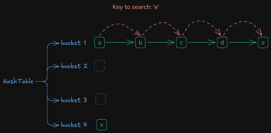
This is where things become interesting because we can finally understand why hash tables lookups are considered O(1) on average. Finding a key in a hash table is such an easy task:

1. calculate hash value of the key to select the bucket
2. loop over the nodes and compare your key with the node key string

For better performance, the hash value of a node is usually stored alongside the key. During lookup, the hash values are compared first, and if they match, the actual keys are compared to confirm equality.

Question: If you have to iterate over the nodes of a bucket’s linked list, why is the lookup complexity considered O(1)?

That’s a very good question.

Assume you have a fixed length array of integers, you are to find a number in this array, what is the time complexity for this search and you would search in linear way? The answer is: O(1) because the you need to check a constant number of value at most. But in the description above, it’s not said that the linked is fixed or any constraint on it. That’s a good point. If we make sure the length of a linked list doesn’t exceed a threshold, we can say that for finding a key on the linked list, a fixed number of iterations is needed. So if the average number of nodes in buckets reach a specific threshold, buckets will be added to hash table.

Strictly speaking, hash table lookups are not always O(1). In the worst case, every key could end up in the same bucket, turning the lookup operation into a linear search with a complexity of O(n). However, with a good hash function and a controlled load factor, keys tend to distribute evenly across buckets. As a result, the average number of nodes that need to be inspected in a bucket remains small and bounded, even as the table grows. This is why hash table operations are commonly described as having average-case O(1) complexity. When the average number of nodes per bucket exceeds a certain threshold, the hash table grows and redistributes its entries across a larger number of buckets.

Deletion

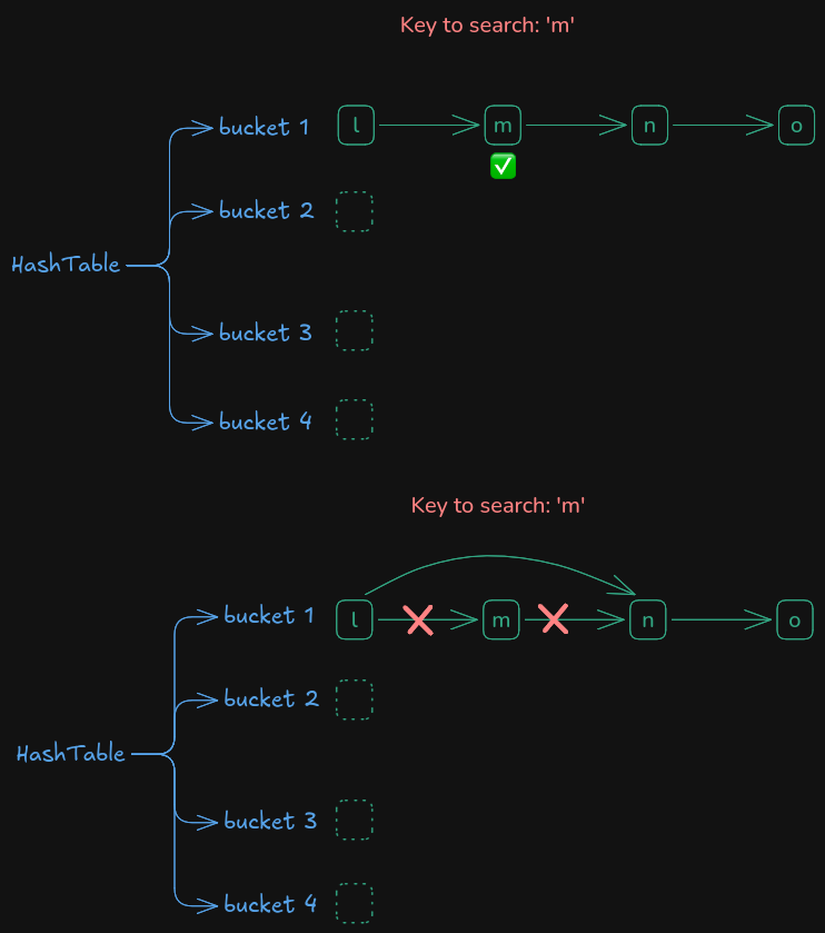
The deletion action is as easy as finding the node in a bucket, if found, connect its previous node to the next node :

Load Factor

The load factor is a measurement of how full a hash table is:

load factor = number of stored keys / number of buckets

As the load factor increases, more keys end up sharing the same buckets, which increases the average lookup cost.

To maintain efficient lookups, hash tables typically resize once the load factor exceeds a predefined threshold. During resizing, a larger bucket array is allocated and existing entries are redistributed across the new buckets.

Collision Resolution

What happens when two different keys are assigned to the same bucket?

This situation is called a collision, and every hash table implementation must handle it somehow.

The approach used in this article is called separate chaining, where each bucket stores a linked list of entries. If multiple keys map to the same bucket, they are simply added to that bucket’s linked list.

Another common strategy is open addressing, where colliding entries are placed into alternative positions inside the bucket array itself. Linear probing, quadratic probing, and double hashing are examples of open-addressing techniques.

For simplicity, our implementation uses separate chaining.

What if keys don’t distribute across buckets evenly?

That’s the case where more iterations are required to find the keys. For example you have 4 buckets initially, and your threshold is 4, and this is your hash table after inserting a couple of keys:

bucket 1 : [a] -> [b] -> [c] -> [d] -> [e] -> [f] -> [g] -> [h] -> [i]
bucket 2 : [j]
bucket 3 : [k]
bucket 4 :

You can easily notice that the problem is there is quite different number of iterations needed to find a key in bucket 1 and other buckets. So what causes this issue?

>»»»»»»»»»» HASH FUNCTION «««««««««««

Aside from the hash function performance, a good hash function is the one that distribute keys as evenly as possible across buckets. One of the most common hash functions is djb2. It’s a non-cryptographic hash function:

 1
 2
 3
 4
 5
 6
 7
 8
 9
10

uint64_t djb2(const char *str)
{
    uint64_t hcode = 5381;
    char ch = 0;
    while ((ch = *str++)) {
        hcode = (hcode << 32) + hcode + ch;
    }

    return hcode;
}

The initial value of hash code is derived experimentally and specified by the author of this function Dan J. Bernstein.

Do you have any guess what the problem is with this hash function? If you have a program that users can input key values and they know you are using a hash function like djb2, they can input data so that only one of the buckets are filled and sabotage your hash table key distribution. You ask me how? Let me explain. Suppose these are the keys and their corresponding hash value generated by our hash function:

If an attacker knows which keys produce which bucket indices, they can intentionally provide inputs that collide into the same bucket. In this example, inputs such as a, f, and k would all end up in bucket 1, while b, g, and l would all end up in bucket 2.

Here’s the scenario that clears the issue:

insertion of 16 values:

bucket 1 : [a] -> [b] -> [c] -> [d] -> [e] -> [f] -> [g] -> [h] -> [i]
bucket 2 : [j]
bucket 3 : [k] -> [l] -> [m] -> [n]
bucket 4 : [o]

size of hash table % buckets count -> 16 / 4 = 4
load_factor(4) >= threshold (4) -> hash table should be extended

Here’s an example that shows the extended buckets after crossing the hash table threshold resize. Existing entries are redistributed across the newly allocated buckets.

bucket 1 : [e] -> [g]
bucket 2 : [j]
bucket 3 : [k] -> [m]
bucket 4 : [o]
bucket 5 : [b] -> [d] -> [f] -> [h] -> [i]
bucket 6 : [a] -> [c]
bucket 7 : [n]
bucket 8 : [l]

Notice that when the number of buckets increases, each key is assigned to a bucket again using the new bucket count:

selected_bucket = hash(key) % 8

As a result, some keys remain in their original buckets while others move to newly created buckets. This redistribution process is called rehashing.

To mitigate collision attacks, many systems introduce randomness into their hashing process or use attack-resistant hash functions. The goal is to make it difficult for an attacker to predict which inputs will collide and degrade hash table performance. Also it’s good to show a good distribution of keys, although there is a bucket in this hash table that has more keys than the load factor value.

bucket 1 : [a] -> [b] -> [c] -> [d]
bucket 2 : [e] -> [f] -> [g] -> [h] -> [i]
bucket 3 : [j] -> [k] -> [l] -> [m]
bucket 4 : [n] -> [o] -> [p] -> [q]
bucket 5 : [r] -> [s] -> [t]
bucket 6 : [u] -> [v] -> [w] -> [x]
bucket 7 : [y]
bucket 8 : [z]

C code for hash table

Why Use a Bit Mask Instead of Modulo?

You may notice that the implementation uses:

1

pos = hash & mask;

instead of;

1

pos = hash % bucket_count;

This optimization works because the number of buckets is always a power of two.

For example, if there are 8 buckets:

bucket_count = 8
mask = 7

which in binary becomes:

8  = 1000
7  = 0111

Applying a bitwise AND with the mask extracts the lower bits of the hash value, producing the same result as a modulo operation while being faster and commonly used in high-performance hash table implementations. Here’s an implementation of hash table in C:

hashtable.h

 1
 2
 3
 4
 5
 6
 7
 8
 9
10
11
12
13
14
15
16
17
18
19
20
21
22
23
24
25
26
27
28
29
30
31
32
33
34
35

#ifndef _HASHTABLE_H
#define _HASHTABLE_H

#include "estring.h"
#include "slist.h"
#include <stddef.h>
#include <stdint.h>

struct HashNode {
    struct HashNode *next;
    uint64_t hcode;
    string_t key;
    string_t value;
};

struct HashNode *node_create(const char *key, const char *val);
void node_free(struct HashNode *node);

struct HashMap {
    struct HashNode **buckets;
    size_t mask;
    size_t size;
};

struct HashTable {
    struct HashMap main;
    struct HashMap temp;
    size_t resizing_pos;
};

void ht_insert(struct HashTable *ht, struct HashNode *node);
struct HashNode *ht_pop(struct HashTable *ht, struct HashNode *node);
struct HashNode *ht_lookup(struct HashTable *ht, struct HashNode *node);

#endif

hashtable.c

  1
  2
  3
  4
  5
  6
  7
  8
  9
 10
 11
 12
 13
 14
 15
 16
 17
 18
 19
 20
 21
 22
 23
 24
 25
 26
 27
 28
 29
 30
 31
 32
 33
 34
 35
 36
 37
 38
 39
 40
 41
 42
 43
 44
 45
 46
 47
 48
 49
 50
 51
 52
 53
 54
 55
 56
 57
 58
 59
 60
 61
 62
 63
 64
 65
 66
 67
 68
 69
 70
 71
 72
 73
 74
 75
 76
 77
 78
 79
 80
 81
 82
 83
 84
 85
 86
 87
 88
 89
 90
 91
 92
 93
 94
 95
 96
 97
 98
 99
100
101
102
103
104
105
106
107
108
109
110
111
112
113
114
115
116
117
118
119
120
121
122
123
124
125
126
127
128
129
130
131
132
133
134
135
136
137
138
139
140
141
142
143
144
145
146
147
148
149
150
151
152
153
154
155
156
157
158
159
160
161
162
163
164
165
166

#include "hashtable.h"
#include "estring.h"
#include "hashfunc.h"
#include "log.h"
#include "slist.h"
#include <assert.h>
#include <stddef.h>
#include <stdio.h>
#include <stdlib.h>
#include <string.h>

const int resize_count = 128;
const int k_max_load_factor = 8;

struct HashNode *node_create(const char *key, const char *val)
{
    assert(key != NULL);
    struct HashNode *node = calloc(1, sizeof(struct HashNode));
    node->hcode = djb2(key);
    node->key = str_from(key);
    if (val)
        node->value = str_from(val);
    return node;
}

void node_free(struct HashNode *node)
{
    str_free(node->key);
    str_free(node->value);
    free(node);
}

static void h_init(struct HashMap *hm, size_t n)
{
    assert((n & (n - 1)) == 0);
    if (!hm) {
        return;
    }
    hm->buckets = calloc(n, sizeof(struct HashNode *));
    hm->mask = n - 1;
    hm->size = 0;
}

static void h_insert(struct HashMap *hm, struct HashNode *node)
{
    size_t pos = node->hcode & hm->mask;
    struct HashNode *next = hm->buckets[pos];
    node->next = next;
    hm->buckets[pos] = node;
    hm->size++;
}

static struct HashNode **h_lookup(struct HashMap *hm, struct HashNode *node)
{
    if (hm->buckets == NULL) {
        warn("hm bucket is null");
        return NULL;
    }
    size_t pos = node->hcode & hm->mask;
    struct HashNode **from = &hm->buckets[pos];
    while (*from) {
        if (node->hcode == (*from)->hcode)
            return from;
        from = &(*from)->next;
    }

    return NULL;
}

static struct HashNode *h_detach(struct HashMap *hm, struct HashNode **from)
{
    struct HashNode *node = *from;
    *from = (*from)->next;
    hm->size--;
    return node;
}


static void ht_resize_init(struct HashTable *ht)
{
    assert(ht->temp.buckets == NULL);
    ht->temp = ht->main;
    h_init(&ht->main, (ht->main.mask + 1) << 1);
    ht->resizing_pos = 0;
}

static void ht_resize(struct HashTable *ht)
{
    if (!ht->temp.buckets)
        return;

    int n = 0;
    struct HashNode **from = ht->temp.buckets;
    while (ht->resizing_pos < ht->temp.mask + 1 && n < resize_count) {
        if (!(*from)) {
            ht->resizing_pos++;
            continue;
        }
        struct HashNode *node = h_detach(&ht->temp, from);
        h_insert(&ht->main, node);
    }
    info("Moved %d keys", n);
}

void ht_insert(struct HashTable *ht, struct HashNode *node)
{
    if (!ht->main.buckets) {
        h_init(&ht->main, 4);
    }

    struct HashNode **from = h_lookup(&ht->main, node);
    if (from) {
        struct HashNode *oldnode = *from;
        *from = node;
        node->next = oldnode->next;
        node_free(oldnode);
    }
    else {
        h_insert(&ht->main, node);
    }

    if (ht->temp.buckets == NULL) {
        int load_factor = ht->main.size / (ht->main.mask + 1);
        if (load_factor >= k_max_load_factor) {
            ht_resize_init(ht);
        }
    }
    else {
        struct HashNode **from = h_lookup(&ht->temp, node);
        if (from) {
            node_free(*from);
        }
    }
    ht_resize(ht);
}

struct HashNode *ht_pop(struct HashTable *ht, struct HashNode *node)
{
    ht_resize(ht);

    struct HashNode **result;
    result = h_lookup(&ht->temp, node);
    if (result) {
        return h_detach(&ht->temp, result);
    }

    result = h_lookup(&ht->main, node);
    if (result) {
        return h_detach(&ht->main, result);
    }

    return NULL;
}

struct HashNode *ht_lookup(struct HashTable *ht, struct HashNode *node)
{
    ht_resize(ht);

    struct HashNode **result = h_lookup(&ht->main, node);
    if (!result) {
        error("looking for node in temp");
        result = h_lookup(&ht->temp, node);
    }

    return result ? *result : NULL;
}

You can inspect the code at: https://github.com/shayaniox/redis